

|  |  | NBAC Tutorial |
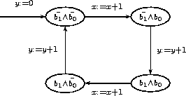
Let us describe a very simle (and maybe stupid) example. We would like to analyse the system depicted on the following figure, where two counters are alternatively incremented.

state
  b0,b1: bool;
  x,y : int;

transition
  b0' = not b1;
  b1' = b0;
  b2' = b2 xor (b0 and b1);
  x' = if (b0 = b1) then x+1 else x;
  y' = if (b0 <> b1) then y+1 else y;

initial not b0 and not b1 and x=0 and y=0;
Here we have state variables, but no input variables, as there is no
interaction with an environment. Suppose now we want to check that x is always greater than or
equal to y. We add the declaration
final not (x>=y);
Actually, for some reasons we will explain later, we prefer to "delay" the initial and final sets of states, using a Boolean variable as follows. This gives the program:
state
  init,ok : bool;
  b0,b1: bool;
  x,y : int;

transition
  init' = false;
  ok' = if init then true else    ok and x>=y;
  b0' = if init then false else   not b1;
  b1' = if init then false else   b0;
  x' = if init then 0 else        if (b0 = b1) then x+1 else x;
  y' = if init then 0 else        if (b0 <> b1) then y+1 else y;
initial init;
final not init and not ok;
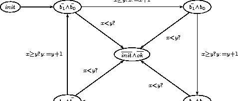
Our system corresponds now to the automaton

Let now ask the tool to perform a step of slicing analysis with the command
nbacg example1.ba -analysis 2 -print "+p +a +r"
The option -analysis 2 indicates we want to perform slicing or
verification, the option -print "+p +a +r" indicates
we want to have information about initial control analysis (+a) and
refinement (+r).
    - Syntaxical analysis
    - Transformation to BDDs
    - Treatement of definition of  - Treatement of equation of ok init y x b1 b0
    - Treatement of formula: assertion initial final
    - Simplification by careset
      Variable reordering done
      Variable reordering done
    - Simplification by Boolean slicing (reach/coreach)
      Variable reordering done
      Forward analysis (.....)
      Backward analysis (..)
      Variable reordering done
    [ v = 0, etiq =  control=!ok^!init; def=(true, 1>=0); cube=true ,
	     succ = [],
	     pred = [2],
      v = 1, etiq =  control=init; def=(true, 1>=0); cube=true ,
	     succ = [2],
	     pred = [],
      v = 2, etiq =  control=ok^!init; def=(true, 1>=0); cube=true ,
	     succ = [0; 2],
	     pred = [1; 2],
      ]
    [ (1,2), bassert=true;
	       cube=true;
	       dec=(0.00 prod, 0.00 ite, 1.00 inter, 1.00 dec) ;
      (2,0), bassert=y>=x+1;
	       cube=y>=x+1;
	       dec=(0.00 prod, 3.00 ite, 1.00 inter, 4.00 dec) ;
      (2,2), bassert=!y>=x+1;
	       cube=!y>=x+1;
	       dec=(0.00 prod, 3.00 ite, 1.00 inter, 4.00 dec) ;
      ]
    (3 vertices, 3 edges, 1.00 e/v, dev(succ/v) = 0.82 dev(pred/v) = 0.82
      postpre : (0.00 prod, 2.00 ite, 1.00 inter, 3.00 dec))
First of all, NBAC parses the input file and transform all
the expressions into BDDs and MTBDDs. It simplifies the formula by taking into account a careset, which represent the knowledge that some numerical constraints implies other ones. Typically, the fact that

is taken into account in the careset.
Then a Boolean slicing is performed: here only the behaviour of Boolean state variables is analysed. Numerical constraints of the involved formula are just viewed as Boolean inputs however constrained by the careset. A partial knowledge about the numerical domain is then taken into account, but in static way: there is no analysis of the dynamic behaviour of numerical variables during an execution at that step.
At last, NBAC build the initial control structure displayed above, with its graphical representation below.

The control structure here is generated by the tool by exactly partitioning the current state space (after Boolean slicing) into initial, final, and other states, and then using a (set of) location(s) to represent each equivalence class. The advantage of using two Boolean variables init and final is to ensure that one location is enough to excatly the set of initial states. Otherwise, we have to decompose these sets in an exact union of abstract values.
Now NBAC performs a first reachability analysis:
    *** Analysis ***
    [ v = 0, etiq =  control=!ok^!init; def=(true, 1>=0); cube=true ,
	     succ = [],
	     pred = [2],
      v = 1, etiq =  control=init; def=(true, 1>=0); cube=true ,
	     succ = [2],
	     pred = [],
      v = 2, etiq =  control=ok^!init; def=(true, 1>=0); cube=true ,
	     succ = [0; 2],
	     pred = [1; 2],                                                           ]
    [ (1,2), bassert=true;
	       cube=true;
	       dec=(0.00 prod, 0.00 ite, 1.00 inter, 1.00 dec) ;
      (2,0), bassert=y>=x+1;
	       cube=y>=x+1;
	       dec=(0.00 prod, 3.00 ite, 1.00 inter, 4.00 dec) ;
      (2,2), bassert=!y>=x+1;
	       cube=!y>=x+1;
	       dec=(0.00 prod, 3.00 ite, 1.00 inter, 4.00 dec) ;                    ]
    (3 vertices, 3 edges, 1.00 e/v, dev(succ/v) = 0.82 dev(pred/v) = 0.82
      postpre : (0.00 prod, 2.00 ite, 1.00 inter, 3.00 dec))
    *** End of analysis in 5 iterations ***
    *** narrowing ***
    *** End narrowing in 1 iterations without stabilization ***
    *** Analysis ***
    [ v = 0, etiq =  control=!ok^!init; def=(true, y>=x,y<=x+2,y+x>=2);
		      cube=true ,
	     succ = [2],
	     pred = [],
      v = 1, etiq =  control=init; def=(true, 1>=0); cube=true ,
	     succ = [],
	     pred = [2],
      v = 2, etiq =  control=ok^!init; def=(true, y>=0,1>=0,y<=x+1,x>=0);
		      cube=true ,
	     succ = [1; 2],
	     pred = [0; 2],
    ]
    [ (0,2), bassert=y>=x+1;
	       cube=y>=x+1;
	       dec=(0.00 prod, 3.00 ite, 1.00 inter, 4.00 dec) ;
      (2,1), bassert=true;
	       cube=true;
	       dec=(0.00 prod, 0.00 ite, 1.00 inter, 1.00 dec) ;
      (2,2), bassert=!y>=x+1;
	       cube=!y>=x+1;
	       dec=(0.00 prod, 3.00 ite, 1.00 inter, 4.00 dec) ;
    ]
    (3 vertices, 3 edges, 1.00 e/v, dev(succ/v) = 0.82 dev(pred/v) = 0.82
     postpre : (0.00 prod, 2.00 ite, 1.00 inter, 3.00 dec))
The initial control structure is displayed once again. After end of analysis and narrowing, the resulting control structure is displayed, however in a transposed way (it is made ready for a backward analysis). Let us depict in graphically in the right orientation:

*** End of analysis in 4 iterations ***
*** narrowing ***
*** End narrowing in 1 iterations with stabilization ***
*** Refinement ***
    [ v = 0, etiq =  control=!ok^!init; def=(true, y>=x,y<=x+2,y+x>=2);
		      cube=true ,
	     succ = [],
	     pred = [2],
      v = 1, etiq =  control=init; def=(true, 1>=0); cube=true ,
	     succ = [2],
	     pred = [],
      v = 2, etiq =  control=ok^!init; def=(true, y<=x+1,1>=0,x>=0,y>=0);
		      cube=true ,
	     succ = [0; 2],
	     pred = [1; 2],
      ]
    [ (1,2), bassert=true;
	       cube=true;
	       dec=(0.00 prod, 0.00 ite, 1.00 inter, 1.00 dec) ;
      (2,0), bassert=y>=x+1;
	       cube=y>=x+1;
	       dec=(0.00 prod, 3.00 ite, 1.00 inter, 4.00 dec) ;
      (2,2), bassert=!y>=x+1;
	       cube=!y>=x+1;
	       dec=(0.00 prod, 3.00 ite, 1.00 inter, 4.00 dec) ;
      ]
    (3 vertices, 3 edges, 1.00 e/v, dev(succ/v) = 0.82 dev(pred/v) = 0.82
      postpre : (0.00 prod, 2.00 ite, 1.00 inter, 3.00 dec))
The analysis didn't bring us new information, so the control structure remains unchanged. So a refinement is needed, in order to improve the precision of the analysis.
    cfc=[[]; [1]; [2]; [0]]
    refine_cfc forward
      vertex 2, mset=[(b1,1); (b0,1); (y>=x+1,3)]
      vertex 0, mset=[]
    result = [2 => y>=x+1;]

    *** Analysis ***
    [ v = 0, etiq =  control=!ok^!init; def=(true, y>=x,y<=x+2,y+x>=2);
		      cube=true ,
	     succ = [],
	     pred = [2],
      v = 1, etiq =  control=init; def=(true, 1>=0); cube=true ,
	     succ = [3],
	     pred = [],
      v = 2, etiq =  control=ok^!init; def=(true, y=x+1,1>=0,y>=1);
		      cube=y>=x+1 ,
	     succ = [0],
	     pred = [3],
      v = 3, etiq =  control=ok^!init; def=(true, y<=x,1>=0,y>=0);
		      cube=!y>=x+1 ,
	     succ = [2; 3],
	     pred = [1; 3],
      ]
    [ (1,3), bassert=true;
	       cube=true;
	       dec=(0.00 prod, 0.00 ite, 1.00 inter, 1.00 dec) ;
      (2,0), bassert=true;
	       cube=true;
	       dec=(0.00 prod, 3.00 ite, 1.00 inter, 4.00 dec) ;
      (3,2), bassert=!b1^b0 + b1^!b0;
	       cube=true;
	       dec=(0.00 prod, 0.00 ite, 1.00 inter, 1.00 dec) ;
      (3,3), bassert=true;
	       cube=true;
	       dec=(0.00 prod, 3.00 ite, 1.00 inter, 4.00 dec) ;                    ]
    (4 vertices, 4 edges, 1.00 e/v, dev(succ/v) = 0.71 dev(pred/v) = 0.71
      postpre : (0.00 prod, 1.50 ite, 1.00 inter, 2.50 dec))

Let us perform a forward analysis:
    *** End of analysis in 5 iterations ***
    *** narrowing ***
    *** End narrowing in 1 iterations with stabilization ***
    *** Analysis ***
    [ v = 0, etiq =  control=!ok^!init; def=(!b1^b0 + b1^!b0, y=x,1>=0,y>=1);
		      cube=!y>=x+1 ,
	     succ = [2],
	     pred = [],
      v = 1, etiq =  control=init; def=(true, 1>=0); cube=true ,
	     succ = [],
	     pred = [3],
      v = 2, etiq =  control=ok^!init; def=(!b1^!b0 + b1^b0, y=x+1,x>=0,1>=0);
		      cube=y>=x+1 ,
	     succ = [3],
	     pred = [0],
      v = 3, etiq =  control=ok^!init; def=(true, y<=x,1>=0,y>=0);
		      cube=!y>=x+1 ,
	     succ = [1; 3],
	     pred = [2; 3],
      ]
    [ (0,2), bassert=!b1^!b0 + b1^b0;
	       cube=true;
	       dec=(0.00 prod, 3.00 ite, 1.00 inter, 4.00 dec) ;
      (2,3), bassert=!b1^b0 + b1^!b0;
	       cube=true;
	       dec=(0.00 prod, 0.00 ite, 1.00 inter, 1.00 dec) ;
      (3,1), bassert=true;
	       cube=true;
	       dec=(0.00 prod, 0.00 ite, 1.00 inter, 1.00 dec) ;
      (3,3), bassert=true;
	       cube=true;
	       dec=(0.00 prod, 3.00 ite, 1.00 inter, 4.00 dec) ;
      ]
    (4 vertices, 4 edges, 1.00 e/v, dev(succ/v) = 0.71 dev(pred/v) = 0.71
      postpre : (0.00 prod, 1.50 ite, 1.00 inter, 2.50 dec))
which can graphically depicted with:

    *** End of analysis in 3 iterations ***
    *** narrowing ***
    *** End narrowing in 1 iterations with stabilization ***
    *** Conclusion ***
    Success automaton
    [ v = 0, etiq =  control=!ok^!init; def=(!b1^b0 + b1^!b0, y=x,1>=0,y>=1);
		      cube=!y>=x+1 ,
	     succ = [],
	     pred = [2],
      v = 2, etiq =  control=ok^!init; def=(!b1^!b0 + b1^b0, y=x+1,x>=0,1>=0);
		      cube=y>=x+1 ,
	     succ = [0],
	     pred = [3],
      v = 3, etiq =  control=ok^!init; def=(!b1^b0 + b1^!b0, y=x,x>=0,1>=0);
		      cube=!y>=x+1 ,
	     succ = [2; 3],
	     pred = [3],
      ]
    [ (2,0), bassert=!b1^!b0 + b1^b0;
	       cube=true;
	       dec=(0.00 prod, 3.00 ite, 1.00 inter, 4.00 dec) ;
      (3,2), bassert=!b1^b0 + b1^!b0;
	       cube=true;
	       dec=(0.00 prod, 0.00 ite, 1.00 inter, 1.00 dec) ;
      (3,3), bassert=true;
	       cube=true;
	       dec=(0.00 prod, 3.00 ite, 1.00 inter, 4.00 dec) ;
      ]
    (3 vertices, 3 edges, 1.00 e/v, dev(succ/v) = 0.82 dev(pred/v) = 0.00
      postpre : (0.00 prod, 2.00 ite, 1.00 inter, 3.00 dec))

At the end, NBAC displays some statistics:
    2 cycles of analysis, 1 refinements, 1 divisions
    Total time spent in verification : 0.18 sec
      Part of it spent in analysis              : 0.14 sec
      Part of it spent in ref. heuristics       : 0.01 sec
      Part of it spent in partition build & ref : 0.03 sec
    Total time spent in post-pre-conditions : 0.09 sec
      make      : 0.00 sec;
      assertion : 0.02 sec;
      apply     : 0.07 sec
    SUCCESS: property proved
    *** END ***
During the refinement process, you can automatically dump the current control structure to a file in DOT format, see graphviz for details.
If we type the command
nbacg example1.ba -analysis 2 -dot "example1.dot +all"and then convert the DOT file into a Poscript file with the following command (part of graphviz package):
dot -Tps example1.dot >example1.pswe get the following file example1.ps. With the option +all, the control structure is dump between every analysis step (here, forward analysis followed by a backward analysis). The final automaton being empty in this case, it is not displayed !
Let us take the same system, but here we want to perform only
reachability analysis. We type the command
nbacg -analysis 0 -o t.ba -print "+a +r -auto 200" example1.ba
The option -analysis 0 means reachability analysis, the
option -print "-auto 200" increase the maximal size of
control structure which are fully displayed. Last the option
-o t.ba indicates that we want to dump the resulting control
structure into the file t.ba, in the same format that the
format of example1.ba. We get:
...

*** Conclusion ***
Valid automaton
[ v = 1, etiq =  control=init; def=(true, 1>=0); cube=true ,
	 succ = [6],
	 pred = [],
  v = 3, etiq =  control=b1^b0^ok^!init; def=(true, y=x,x>=1,1>=0);
		  cube=!y>=x+1 ,
	 succ = [5],
	 pred = [4],
  v = 4, etiq =  control=!b1^b0^ok^!init; def=(true, y+1=x,x>=1,1>=0);
		  cube=!y>=x+1 ,
	 succ = [3],
	 pred = [6],
  v = 5, etiq =  control=b1^!b0^ok^!init; def=(true, y+1=x,x>=2,1>=0);
		  cube=!y>=x+1 ,
	 succ = [6],
	 pred = [3],
  v = 6, etiq =  control=!b1^!b0^ok^!init; def=(true, y=x,1>=0,y>=0);
		  cube=!y>=x+1 ,
	 succ = [4],
	 pred = [1; 5],
  ]
[ (1,6), bassert=true;
	   cube=true;
	   dec=(0.00 prod, 0.00 ite, 1.00 inter, 1.00 dec) ;
  (3,5), bassert=true;
	   cube=true;
	   dec=(0.00 prod, 0.00 ite, 1.00 inter, 1.00 dec) ;
  (4,3), bassert=true;
	   cube=true;
	   dec=(0.00 prod, 0.00 ite, 1.00 inter, 1.00 dec) ;
  (5,6), bassert=true;
	   cube=true;
	   dec=(0.00 prod, 0.00 ite, 1.00 inter, 1.00 dec) ;
  (6,4), bassert=true;
	   cube=true;
	   dec=(0.00 prod, 0.00 ite, 1.00 inter, 1.00 dec) ;
  ]
(5 vertices, 5 edges, 1.00 e/v, dev(succ/v) = 0.00 dev(pred/v) = 0.63
  postpre : (0.00 prod, 0.00 ite, 1.00 inter, 1.00 dec))
3 cycles of analysis, 3 refinements, 4 divisions
Total time spent in verification : 0.26 sec
  Part of it spent in analysis              : 0.11 sec
  Part of it spent in ref. heuristics       : 0.04 sec
  Part of it spent in partition build & ref : 0.11 sec
Total time spent in post-pre-conditions : 0.17 sec
  make      : 0.00 sec;
  assertion : 0.06 sec;
  apply     : 0.11 sec
FAILURE: property not proved
*** OUTPUT ***
Resulting automaton printed to the file t.ba
*** END ***
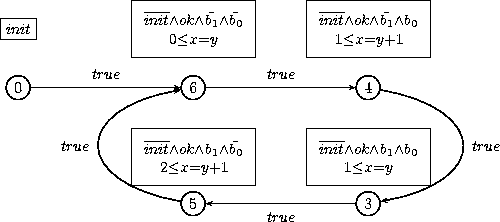
Here the control structure will be refined as long as the heuristics find refinement criteria, then it stops the analysis. There is no verification goal here, so even once final locations are not reachable any more, the process is still continued. The resulting control structure can be graphically depicted:

If we append the option(s) -dot "example1_reach.dot +all", and we translate to Postscript with dot -Tps example1_reach.dot >example1_reach.ps, we get this.
As mentioned above, the resulting control structure, after analysis, can be dumped with the -o t.ba option. Unless the option +success is set and the verification goal is proved, the resulting control structure is dumped to the file t.ba:
state
  b1, b0, ok, init : bool;
  y, x : int;

local
  _cond0, _cond2, _cond4, _cond6, _cond8 : bool;
  _bdd5, _bdd14, _bdd9, _bdd6, _bdd3, _bdd2, _bdd10, _bdd1, _bdd0, _bdd11,
      _bdd12, _bdd7, _bdd4, _bdd13, _bdd8 : bool;
  _int14, _int11, _int12, _int0, _int3, _int13, _int8, _int1, _int9, _int5,
  _int2, _int6, _int4, _int7, _int10 : int;

definition
  _cond0 = b1;
  _cond2 = b0;
  _cond4 = ok;
  _cond6 = init;
  _cond8 = y>=x+1;
  _bdd5 = if b1 then _bdd0 else _bdd3;
  _bdd14 = if b1 then _bdd0 else _bdd12;
  _bdd9 = if b0 then _bdd8 else _bdd0;
  _bdd6 = if ok then _bdd0 else _bdd3;
  _bdd3 = if init then _bdd0 else not _bdd0;
  _bdd2 = if init then _bdd0 else not _bdd1;
  _bdd10 = if b1 then _bdd9 else _bdd0;
  _bdd1 = if _cond8 then _bdd0 else not _bdd0;
  _bdd0 = true;
  _bdd11 = if b1 then _bdd0 else _bdd9;
  _bdd12 = if b0 then _bdd0 else _bdd8;
  _bdd7 = if init then _bdd0 else _bdd1;
  _bdd4 = if b0 then _bdd3 else _bdd0;
  _bdd13 = if b1 then _bdd12 else _bdd0;
  _bdd8 = if ok then _bdd7 else _bdd0;
  _int14 = if b1 then _int12 else _int13;
  _int11 = if init then _int0 else _int10;
  _int12 = if b0 then _int9 else _int11;
  _int0 = 0;
  _int3 = y+1;
  _int13 = if b0 then _int11 else _int9;
  _int8 = x+1;
  _int1 = y;
  _int9 = if init then _int0 else _int8;
  _int5 = if b0 then _int2 else _int4;
  _int2 = if init then _int0 else _int1;
  _int6 = if b0 then _int4 else _int2;
  _int4 = if init then _int0 else _int3;
  _int7 = if b1 then _int5 else _int6;
  _int10 = x;

transition
  ok' = _bdd2;
  init' = not _bdd0;
  y' = _int7;
  x' = _int14;
  b1' = not _bdd4;
  b0' = not _bdd5;
assertion _bdd6;
initial _bdd3;
final not _bdd6;
automaton
  location init0 : _bdd3;
  location good0_n8_b1_b0 : not _bdd10;
  location good0_n8_not_b1_b0 : not _bdd11;
  location good0_n8_b1_not_b0 : not _bdd13;
  location good0_n8_not_b1_not_b0 : not _bdd14;
  edge (init0,good0_n8_not_b1_not_b0) : _bdd0;
  edge (good0_n8_b1_b0,good0_n8_b1_not_b0) : _bdd0;
  edge (good0_n8_not_b1_b0,good0_n8_b1_b0) : _bdd0;
  edge (good0_n8_b1_not_b0,good0_n8_not_b1_not_b0) : _bdd0;
  edge (good0_n8_not_b1_not_b0,good0_n8_not_b1_b0) : _bdd0;
Doesn't look pretty, isn't it ? This is because we want to keep the concise form of the internal BDDs/MTBDDs representation. Each reachable BDD/MTBDD node is declared as a local variable and defined either as a leaf or as a decision node. This textual format can be replace by Disjunctive Normal Forms by using the option -o "-bdd" instead of the default -o "+bdd". Another difference with the initial file is the automaton section, which defines an explicit control structure.
The file t.ba is a valid input to NBAC.
For instance, we can type
nbacg -analysis 1 t.ba -o t2.ba
to perform a coreachability analysis after this reachability analysis.
There is a way to prevent NBAC to refine too much the control structure. If we type
nbacg -analysis 0 -o t.ba -partition "-maxloc 4" example1.ba
we ask NBAC to stop refinement as soon as the current control
structure has at last 4 locations.
Conversely, if we want to perform a coreachability analysis, which compute the set of states that may lead to a final state, we type the command nbacg -analysis 1 -o t.ba -dot "example1_coreach.dot +all" example1.ba and we obtain this.

|  |  | NBAC Tutorial |